Vjeux

I recently had the chance to do a 2-hour Javascript evangelism talk at Dassault Systèmes. Unfortunately the presentation has not been recorded. I reused my the presentation I did at EPITA at the beginning and added a second part with a lot of demos. I've written down notes about the second part so you can get an idea.

Developer Tools

• Web Inspector. It is integrated into Google Chrome and has all the features you would be expecting in an IDE. The console is really powerful as it lets you browse through the Javascript objects. You no longer need to write endless printing functions. You can edit the HTML and CSS without a page reload, it makes designing interfaces a lot more efficient. There is also a full panel dedicated to profiling both Javascript and DOM events.
• JSFiddle. Web programming is all about interactivity. Not only you with the program (REPL) but also with other people. Everything you do can be one link away. JSFiddle lets you try and experiment things without the need of an IDE and allows you to show it to the world easily.
• JSHint. Because Javascript, the language, has design issues and is highly dynamic, it is useful to enforce good practices and to set common programming rules when working together. Always in the spirit of the web, you can just copy and paste your code to check it. Note that JSHint can also be integrated in all major text editors and IDEs.

CSS

HTML and CSS were traditionally used to make websites and forms. We can now make completely different things.

• jmpress.js. Here's an example of how to use 3D in CSS in order to make animated presentation. One important thing to notice is how easy it is to use it. Just include jmpress.js in the page and add data-x="-5000" data-rotate="180" attributes to your HTML. It just works!
• CSS Panic. In order to show how powerful CSS got those days, here's a game completely written in HTML + CSS. There is 0 lines of Javascript!

Canvas

Canvas is just a rectangle where you can manipulate each pixel's color.

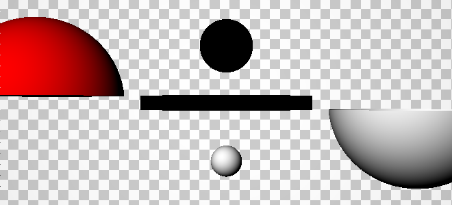
• RayTracer. Ray Tracer is a common computer science school project. Usually, you write it on your computer and sometimes share the resulting image but you don't really share it because no one want to take the pain of compiling it on their machine. With Javascript, you can just share a link and everyone can test it!
• Canvas Rider. You can now create games in the browser. There is even a level editor implemented that follows principle of the web: interactivity. You can draw the map and move your character at the same time. When you are done, you are a single click away from saving the map and sharing it to people.
• pdf.js. The browser is now able to create applications that have always been restricted to native ones. The perfect example is this demo by Mozilla of a pdf renderer written exclusively in Javascript!

SVG

SVG let you manipulate vector graphics such as line, curve, circle ...

• Cloth Simulation. Javascript implementations have gotten fast enough to do real time constraint solving simulations such as this one. It uses SVG to easily render the graph.
• Simulated Annealing. It's another school project that gains from being written in the web. This would have probably been written in console mode, using ascii art and generating images as output. The parameters would have been entered in the command line. We can instead exploit HTML to make forms that update in real time, and SVG to render the problem and a graph to display the progress.

WebGL

WebGL is an implementation of OpenGL in the browser. It let us use the graphical card from Javascript.

• 3D Simulated Annealing. Same as previous demo but this time there is a 3D representation of the progress. It also follows the interactivity rule, you can use your mouse and WASD to explore the scene. This demo uses Web Workers to exploit multiple cores.
• WebGL Maps. The graphical card is dedicated to manipulate images, therefore you can use it to improve performance on image intensive applications such as Google Maps.
• Bevelity. Ever wondered if it was possible to write a complex application such as 3DSMax in the browser? Bevelity is an attempt to prove it true.
• Water Simulation. Another physics simulation demo with always the web plus: you can move the ball 🙂
• Hello Racer. This is one of the thousand demos that shows you a beautiful car with glossy reflects ... This one has a unique feature: you can move the car! This must not have taken more than a few dozens of lines and yet has a huge impact!
• Morph Target. Pixar also find uses for the web. Here's a demo to create facial expressions.
• Rome. Browsers now embed a video tag. Using it in combination with WebGL, Google made a wonderful 3-minute animation. You can use the mouse to interact with it. It moves the camera, pixelate the video and even make appear various monsters.

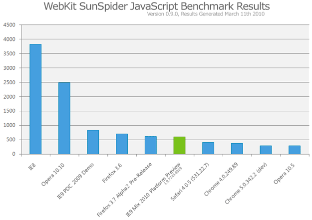
Performance

Javascript performance are impressively improving from months to months. It is now possible to write computing intensive programs and make them run at decent speed.

• JSPerf. If you have a doubt on which browser is faster for a specific feature or when you have two ways to do things, which one is faster, JSPerf is made for you!
• JSLinux. Typed Arrays introduced for WebGL made possible to write a CPU Virtual Machine able to run a copy of linux in under 7 seconds.
• repl.it. Emscriptem is a wonderful tool that translates LLVM assembly code into Javascript. It made possible to compile Ruby, Python, Lua and Scheme directly from their sources to Javascript.
• Broadway. Last but not least, a H.264 video decoder has been compiled to Javascript using Emscriptem. It manages to decode the sample videos at 60 frames per second. This is an exceptional feat for a scripting language!

Conclusion

It is now possible to write the same complex applications we seen in the past in the browser. And it gives one huge added value: interactivity. There's absolutely nothing to install, you just have to give a link! You can combine all the render options such as HTML, CSS, Canvas, SVG and WebGL to make your program.

The next talk I'm going to do is at the JSConf! I hope to see you there!

Here is a report of the Ray Tracer written by myself Christopher Chedeau. I've taken the file format and most of the examples from the Ray Tracer of our friends Maxime Mouial and Clément Bœsch. The source is available on Github.

It is powered by Open Source technologies: glMatrix, CodeMirror, CoffeeScript, Twitter Bootstrap, jQuery and Web Workers.

Check out the demo, or click on any of the images.

Objects

Our Ray Tracer supports 4 object types: Plane, Sphere, Cylinder and Cone.

The core idea of the Ray Tracer is to send rays that will be reflected on items. Given a ray (origin and direction), we need to know if it intersect an object on the scene, and if it does, how to get a ray' that will be reflected on the object.

Knowing that, we open up our high school math book and come up with all the following formulas.

Legend: Ray Origin \(O\), Ray Direction \(D\), Intersection Position \(O'\), Intersection Normal \(N\) and Item Radius \(r\).

In order to solve the equation \(at^2 + bt + c = 0\), we use
\[\Delta = b^2 - 4ac \]\[
\begin{array}{c c c}
\Delta \geq 0 & t_1 = \frac{-b - \sqrt{\Delta}}{2a} & t_2 = \frac{-b + \sqrt{\Delta}}{2a}
\end{array}
\]

And here is the formula for the reflected ray:

\[
\left\{
\begin{array}{l}
O' = O + tD + \varepsilon D' \\
D' = D - 2 (D \cdot N) * N
\end{array}
\right.
\]

In order to fight numerical precision errors, we are going to move the origin of the reflected point a little bit in the direction of the reflected ray (\(\varepsilon D'\)). It will avoid to falsely detect a collision with the current object.

Coordinates, Groups and Rotations

We want to move and rotate objects. In order to do that, we compute a transformation matrix (and it's inverse) for each object in the scene using the following code:

\[
T = \begin{array}{l}
(Identity * Translate_g * RotateX_g * RotateY_g * RotateZ_g) * \\
(Identity * Translate_i * RotateX_i * RotateY_i * RotateZ_i)
\end{array}
\]\[ I = T^{-1} \]

We have written the intersection and normal calculations in the object's coordinate system instead of the world's coordinate system. It makes them easier to write. We use the transformation matrix to do object -> world and the inverse matrix to do world -> object.

Bounding Box

The previous equations give us objects with infinite dimensions (except for the sphere) whereas objects in real life have finite dimensions. To simulate this, it is possible to provide two points that will form a bounding box around the object. On the intersection test, we are going to use the nearest point that is inside the bounding box.

This gives us the ability to do various objects such as mirrors, table surface and legs, light bubbles and even a Pokeball!

Light

An object is composed of an Intensity \(I_o\), a Color \(C_o\) and a Brightness \(B_o\). Each light has a Color \(C_l\) and there is an ambient color \(C_a\). Using all those properties, we can calculate the color of a point using the following formula:

\[
I_o * (C_o + B_o) * \left(C_a + \sum_{l}{(N \cdot D) * C_l}\right)
\]

Only the lights visible from the intersection point are used in the sum. In order to check this, we send a shadow ray from the intersection point to the light and see if it intersects any object.

The following images are examples to demonstrate the lights.

Textures

In order to put a texture on an object, we need to map a point \((x, y, z)\) in the object's coordinate system into a point \((x, y)\) in the texture's coordinate system. For planes, it is straightforward, we just the \(z\) coordinate (which is equal to zero anyway). For spheres, cylinders and cones it is a bit more involved. Here is the formula where \(w\) and \(h\) are the width and height of the texture.

\[
\begin{array}{c c}
\phi = acos(\frac{O'_y}{r}) & \theta = \frac{acos\left(\frac{O'_x}{r * sin(\phi)}\right)}{2\pi}
\end{array}
\]\[
\begin{array}{c c}
x = w * \left\{\begin{array}{l l} \theta & \text{if } O'_x < 0 \\ 1 - \theta & \text{else}\end{array}\right. & y = h * \frac{\phi}{\pi} \end{array} \] Once we have the texture coordinates, we can easily create a checkerboard or put a texture. We added options such as scaling and repeat in order to control how the texture is placed.

We also support the alpha mask in order to make a color from a texture transparent.

Progressive Rendering

Ray tracing is a slow technique. At first, I generated pixels line by line, but I found out that the first few lines do not hold much information.

Instead, what we want to do is to have a fast overview of the scene and then improve on the details. In order to do that, during the first iteration we are only generating 1 pixel for a 32x32 square. Then we generate 1 pixel for a 16x16 square and so on ... We generate the top-left pixel and fill all the unknown pixels with it.

In order not to regenerate pixels we already seen, I came up with a condition to know if a pixel has already been generated. \(size\) is the current square size (32, 16, ...).

\[\left\{\begin{array}{l}
x \equiv 0 \pmod{size * 2}\\
y \equiv 0 \pmod{size * 2}
\end{array}\right.
\]

Supersampling

Aliasing is a problem with Ray Tracing and we solve this issue using supersampling. Basically, we send more than one ray for each pixel. We have to chose representative points from a square. There are multiple strategies: in the middle, in a grid or random. Check the result of various combinations in the following image:

• 1x: Basic
• 4x: 4 random 1 fixed, 3 random 2x upscale
• 16x: 4x upscale 2x upscale, 1 fixed, 3 random

Perlin Noise

We can generate random textures using Perlin Noise. We can control several parameters such as \(octaves\), the number of basic noise, the initial scale \(f\) and the factor of contribution \(p\) of the high frequency noises.

\[ noise(x, y, z) = \sum_{i = 0}^{octaves}{p^i * PerlinNoise(\frac{2^i}{f}x, \frac{2^i}{f}y, \frac{2^i}{f}z)} \]

As seen in the example, we can apply additional functions after the noise has been generated to make interesting effects.

Portal

Last but not least, Portals from the self-titled game. They are easy to reproduce in a Ray Tracer and yet, I haven't seen any done.

If a ray enters portal A, it will go out from portal B. It is trivial to implement it, it is just a coordinates system transformation. Like we did for world and object transformation, we do it between A and B using their transformation matrix.

Scene Editor

In order to create scenes more easily, we have defined a scene description language. We developed a basic CodeMirror syntax highlighting script. Just enter write your scene down and press Ray Trace 🙂

I've been working on code that works on Browser, Web Workers and NodeJS. In order to export my module, I've been writing ugly code like this one:

(function () {
  /* ... Code that defines MyModule ... */
 
  var all;
  if (typeof self !== 'undefined') {
    all = self; // Web Worker
  } else if (typeof window !== 'undefined') {
    all = window; // Browser
  } else if (typeof global !== 'undefined') {
    all = global; // NodeJS
  }
  all.MyModule = MyModule;
 
  if (typeof module !== 'undefined') {
    module.exports = MyModule;
  }
})();

One-line Solution

Guillaume Marty showed me that sink.js uses this as a replacement for self, window and global. I managed to add support for module.exports in a one-liner!

(function (global) {
  /* ... Code that defines MyModule ... */
 
  global.MyModule = (global.module || {}).exports = MyModule;
})(this);

I have been looking for this magic line for a long time, I hope it will be useful to you too 🙂

For a school project, I have to implement Simulated Annealing meta heuristic.

Thanks to many open source web tools, I've been able to quickly do the project and have a pretty display. CoffeeScript, Raphael, Highcharts, Three.js, Twitter Bootstrap, jQuery and Web Workers.

2D Demo

You have a shuffled grid and you have to find the original grid. The only operation available is to swap 2 random elements. The cost function is the distance of the point with their original neighbors.

Click to view the 2D demo

3D Demo

On this one, we are given many functions and we have to find the global minimum. The challenge was to be able to display the evolution of the algorithm, as it traverses 200k points per second.

Click to view the 3D demo

CoffeeScript Sexyness

I've written the project in CoffeeScript and I don't regret it. I find myself writing code a lot faster because I have a lot less to type. Most of the Javascript syntax is either shortened (function to ->) or optional (parenthesis, curly brackets ...) in CoffeeScript. There are also handy features such as splats, generators ...

Destructuring Assignment

worker.onmessage = (data: [id, rest...]) ->
  switch id
    when 'update'
      [cost, temperature, accepted, tried, data, force] = rest

Trimmed JSON

chart = new Highcharts.Chart
  chart:
    renderTo: 'container'
  yAxis: [
    title:
      text: 'Cost'
  ]
  tooltip:
    formatter: ->
      this.series.name + ': ' + this.y

Report

Felix Abecassis wrote a report that explains everything 🙂 It's in French, sorry!

Download PDF

6 months ago, I wrote the blog post "JSPP - Morph C++ into Javascript". My supervisor at the LRDE (R&D Lab of EPITA), Didier Verna, found it interesting and told me that it could be worth a publication. With his great help, I've written my first article. We have submitted it to two conferences (one after the other) and received two refusals.

• Dynamic Language Symposium (DLS) 2012.
• OOPS 2012: 26th ACM Symposium on Applied Computing. Special track on Object Oriented Programming Languages and Systems.

Overall, the reviewers said the article was well written and the implementation interesting but since it has no practical use, it does not deserve a publication.

Even if it didn't make it, I'm really proud of the article. If you are interested in the implementation of JSPP, it can be an enlightening read 🙂

Download PDF

(For copyright issue, this is not the submitted version of the file. There are still some minor wording issues)